Minimum Spanning Tree with Prim's Algorithm: Python, Java & C++

Navigating the complexities of graph theory is a fundamental skill for any aspiring developer or computer science student. Among the most crucial problems in this domain is finding a Minimum Spanning Tree (MST). This tutorial will thoroughly explore how to implement the minimum spanning tree using Prim's algorithm in Python, Java, and C++, equipping you with a robust understanding and practical coding skills. We will delve into the algorithm's mechanics, its practical applications, and provide step-by-step code examples in three popular programming languages, ensuring you can apply this powerful concept across various development environments. Mastering Prim's algorithm is key to efficiently solving a wide range of network optimization problems, making it an invaluable addition to your algorithmic toolkit.

What is a Minimum Spanning Tree (MST)?
Understanding Prim's Algorithm
Prerequisites
Implementing Minimum Spanning Tree using Prim's Algorithm in Python, Java, and C++
Time and Space Complexity Analysis
- Time Complexity
- Space Complexity
Common Mistakes and How to Avoid Them
Conclusion
Frequently Asked Questions
Further Reading & Resources

What is a Minimum Spanning Tree (MST)?

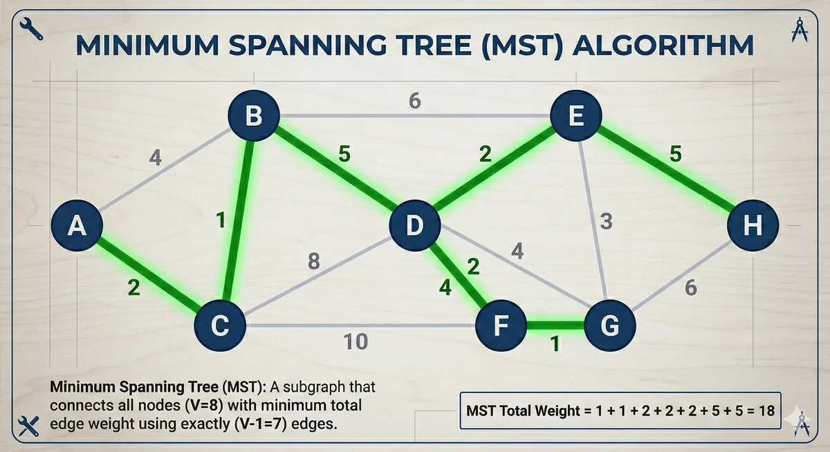
Before diving into Prim's algorithm, let's establish a clear understanding of what a Minimum Spanning Tree is. A graph consists of vertices (nodes) and edges (connections between nodes). A spanning tree of an undirected, connected, and weighted graph is a subgraph that connects all the vertices together, without any cycles, and uses the minimum possible number of edges (specifically, V-1 edges for a graph with V vertices).

A Minimum Spanning Tree takes this concept further by adding the element of edge weights. If each edge in the graph has a numerical weight associated with it (e.g., representing distance, cost, or time), an MST is a spanning tree where the sum of the weights of all its edges is minimized. In essence, it's the "cheapest" way to connect all vertices without forming any loops. MSTs are crucial in many real-world scenarios, from designing efficient network layouts to optimizing transportation routes and even in clustering analysis for data science. For related problems focusing on finding shortest paths within a graph, you might explore algorithms like Dijkstra's Algorithm or Bellman-Ford Algorithm.

Understanding Prim's Algorithm

Prim's algorithm is a greedy algorithm used to find a Minimum Spanning Tree for a weighted undirected graph. A greedy algorithm makes the locally optimal choice at each stage with the hope of finding a global optimum. Prim's algorithm operates by building the MST one edge at a time, starting from an arbitrary vertex.

The core idea is simple: begin with a single vertex, and then iteratively add the cheapest edge that connects a vertex already in the growing MST to a vertex not yet in the MST. This process continues until all vertices are included in the spanning tree. At each step, Prim's algorithm selects the smallest weight edge that expands the tree without creating a cycle, thereby guaranteeing that the total weight of the chosen edges will be minimized. This makes it an efficient and intuitive method for constructing an MST.

How Prim's Algorithm Works: A Step-by-Step Breakdown

To effectively implement Prim's algorithm, it's essential to understand its systematic approach. The algorithm maintains a set of vertices already included in the MST and, at each step, selects an edge that connects a vertex in this set to a vertex outside it, ensuring that the selected edge has the minimum possible weight.

Algorithm Steps for Prim's

Here are the detailed steps for Prim's algorithm, which we will follow in our implementations:

Initialize Data Structures: We need a way to keep track of key information. This typically involves:
- key array (or distance array): Stores the minimum weight of an edge connecting a vertex to the current MST. Initialize key[source_vertex] = 0 and key[other_vertices] = infinity.
- parent array: Stores the parent of each vertex in the MST. This helps reconstruct the tree. Initialize parent[source_vertex] = -1 (or null).
- inMST array (or visited set): A boolean array to mark whether a vertex is already included in the MST. Initialize all to false.
- Adjacency List: Represents the graph efficiently, storing neighbors and edge weights for each vertex.
Choose a Starting Vertex: Select an arbitrary vertex to start building the MST. It doesn't matter which one you pick; the algorithm will find the same MST (assuming the graph is connected). For simplicity, we often choose vertex 0. Set its key to 0.
Iterate to Build the MST: Repeat the following V (number of vertices) times:
Extract the Minimum Key Vertex: From the set of vertices not yet included in the MST (i.e., inMST[v] == false), select the vertex u that has the minimum key value. This vertex u is the next one to be added to the MST. A priority queue is an ideal data structure for efficiently finding this minimum-key vertex.
Add Vertex to MST: Mark u as inMST[u] = true. This signifies that u is now part of our growing Minimum Spanning Tree.
Update Neighbors' Key Values: For each neighbor v of u (i.e., for every edge (u, v) with weight w):
- If v is not yet in the MST (inMST[v] == false) AND the edge weight w is less than the current key[v] value:
  - Update key[v] = w.
  - Set parent[v] = u.
  - If using a priority queue, update v's priority or add v with its new key.
Reconstruct the MST: Once the loop finishes, the parent array will contain the structure of the MST. Each (v, parent[v]) forms an edge in the MST, except for the starting vertex which has parent as -1. The sum of all key[v] values (excluding the initial 0 for the source) gives the total weight of the MST.

Illustrative Example: Step-by-Step Prim's Execution

Let's walk through a simple example to solidify your understanding. Consider a graph with 4 vertices (A, B, C, D) and the following edges:

(A, B) weight 1
(A, C) weight 3
(B, C) weight 1
(B, D) weight 5
(C, D) weight 2

We'll use vertex A as our starting point.

Initial State:

key: [A:0, B:∞, C:∞, D:∞]
parent: [A:-1, B:-1, C:-1, D:-1]
inMST: [A:F, B:F, C:F, D:F]
PriorityQueue: [(0, A, None)]

Iteration 1:

Extract (0, A, None) from PQ. A is not in MST.
Mark inMST[A] = True. Total cost: 0. Add A to MST.
Neighbors of A:
- B (weight 1): inMST[B] is False, 1 < key[B] (∞). Update key[B]=1, parent[B]=A. Add (1, B, A) to PQ.
- C (weight 3): inMST[C] is False, 3 < key[C] (∞). Update key[C]=3, parent[C]=A. Add (3, C, A) to PQ. PriorityQueue: [(1, B, A), (3, C, A)]

Iteration 2:

Extract (1, B, A) from PQ. B is not in MST.
Mark inMST[B] = True. Total cost: 0 + 1 = 1. Add edge (A, B, 1) to MST.
Neighbors of B:
- A (weight 1): inMST[A] is True. Skip.
- C (weight 1): inMST[C] is False, 1 < key[C] (3). Update key[C]=1, parent[C]=B. Add (1, C, B) to PQ. (Note: A new, better path to C found!)
- D (weight 5): inMST[D] is False, 5 < key[D] (∞). Update key[D]=5, parent[D]=B. Add (5, D, B) to PQ. PriorityQueue: [(1, C, B), (3, C, A), (5, D, B)] (PQ will sort by weight, so (1, C, B) is next)

Iteration 3:

Extract (1, C, B) from PQ. C is not in MST.
Mark inMST[C] = True. Total cost: 1 + 1 = 2. Add edge (B, C, 1) to MST.
Neighbors of C:
- A (weight 3): inMST[A] is True. Skip.
- B (weight 1): inMST[B] is True. Skip.
- D (weight 2): inMST[D] is False, 2 < key[D] (5). Update key[D]=2, parent[D]=C. Add (2, D, C) to PQ. PriorityQueue: [(2, D, C), (3, C, A), (5, D, B)] (The older (3, C, A) and (5, D, B) are now redundant but will be skipped when extracted)

Iteration 4:

Extract (2, D, C) from PQ. D is not in MST.
Mark inMST[D] = True. Total cost: 2 + 2 = 4. Add edge (C, D, 2) to MST.
Neighbors of D:
- B (weight 5): inMST[B] is True. Skip.
- C (weight 2): inMST[C] is True. Skip. All vertices are now in MST.

Final MST:

Edges: (A, B, 1), (B, C, 1), (C, D, 2) Total Weight: 4

This detailed walkthrough helps to illustrate how Prim's algorithm systematically builds the MST by always picking the locally cheapest, valid edge.

Prerequisites

To get the most out of this tutorial and successfully implement Prim's algorithm, you should have:

Basic Understanding of Graph Theory: Familiarity with concepts like vertices, edges, weights, connected graphs, and cycles. For examples of other graph traversal problems, consider learning about the CSES Labyrinth Problem.
Data Structure Knowledge: A good grasp of adjacency lists (or matrices), arrays, and especially priority queues (min-heaps).
Programming Fundamentals: Basic to intermediate programming skills in at least one of Python, Java, or C++, including loops, conditional statements, and custom classes/structs.
Object-Oriented Programming (for Java/C++): Understanding how to define and use classes and objects will be beneficial for representing graph edges or nodes.

Implementing Minimum Spanning Tree using Prim's Algorithm in Python, Java, and C++

Let's dive into the practical implementation of Prim's algorithm in our chosen languages. We will use an adjacency list to represent the graph and a priority queue to efficiently select the next minimum-weight edge.

Implementation in Python

Python's heapq module provides a min-heap implementation, which is perfect for our priority queue needs. We'll represent the graph using an adjacency list where each entry stores tuples of (weight, neighbor).

1. Representing the Graph

We'll use a dictionary of lists for the adjacency list. graph[u] will contain (weight, v) for all neighbors v of u.

2. Initializing Data Structures

We'll need min_heap (priority queue), visited set, min_cost_so_far for total MST weight, and a list to store MST edges.

3. Prim's Algorithm Function

The main function will initialize the heap with a starting vertex and then iteratively extract the minimum edge.

import heapq

def prim_mst_python(graph):
    """
    Finds the Minimum Spanning Tree (MST) of a weighted undirected graph
    using Prim's algorithm.

    Args:
        graph (dict): A dictionary representing the adjacency list of the graph.
                      Each key is a vertex, and its value is a list of tuples
                      (weight, neighbor). Example: {0: [(1, 1), (2, 4)], ...}

    Returns:
        tuple: A tuple containing:
            - float: The total minimum cost of the MST.
            - list: A list of tuples (u, v, weight) representing the edges in the MST.
    """
    if not graph:
        return 0, []

    # Choose an arbitrary starting vertex (e.g., the first one in the graph keys)
    start_node = next(iter(graph)) 

    # Priority queue stores tuples: (weight, current_vertex, parent_vertex)
    # The parent_vertex is None for the start_node itself.
    min_heap = [(0, start_node, None)] 

    # Set to keep track of visited nodes (nodes included in the MST)
    visited = set()

    # List to store the edges of the MST
    mst_edges = []

    # Total cost of the MST
    min_cost = 0

    while min_heap and len(visited) < len(graph):
        # Extract the edge with the minimum weight
        weight, u, parent = heapq.heappop(min_heap)

        # If the vertex is already visited, skip it (this handles duplicate entries in heap)
        if u in visited:
            continue

        # Mark the current vertex as visited (add it to the MST)
        visited.add(u)
        min_cost += weight

        # Add the edge to our MST if it's not the starting node's initial entry
        if parent is not None:
            mst_edges.append((parent, u, weight))

        # Explore neighbors of the newly added vertex 'u'
        for edge_weight, v in graph.get(u, []):
            if v not in visited:
                # Add neighbor to the priority queue. The current vertex 'u' is its parent.
                heapq.heappush(min_heap, (edge_weight, v, u))

    # Check if all vertices were included (graph might be disconnected)
    if len(visited) != len(graph):
        # If not all vertices are visited, the graph is disconnected,
        # and a single MST cannot be formed.
        print("Warning: Graph is disconnected. MST found for connected component only.")

    return min_cost, mst_edges

#### 4. Example Usage in Python

```python
# Example graph representation (adjacency list)
# {vertex: [(weight, neighbor), ...]}
graph_python_simple = {
    0: [(4, 1), (8, 7)],
    1: [(4, 0), (8, 2), (11, 7)],
    2: [(8, 1), (7, 3), (2, 5), (4, 8)],
    3: [(7, 2), (9, 4), (14, 5)],
    4: [(9, 3), (10, 5)],
    5: [(2, 2), (14, 3), (10, 4), (1, 6)],
    6: [(2, 7), (6, 8), (1, 5)],
    7: [(8, 0), (11, 1), (7, 8), (2, 6)],
    8: [(4, 2), (7, 7), (6, 6)]
}


cost_py, mst_py = prim_mst_python(graph_python_simple)
print(f"Python MST Cost: {cost_py}")
print("Python MST Edges:")
for u, v, w in mst_py:
    print(f"  ({u}, {v}) - Weight: {w}")

Implementation in Java

In Java, we'll create a custom Edge class to store target vertex and weight. The graph will be an ArrayList of ArrayList<Edge>. Java's PriorityQueue will be used for the min-heap.

1. Representing the Graph

We'll define an Edge class to make graph representation clear. The graph itself will be an ArrayList of ArrayList<Edge>.

import java.util.*;

// Helper class to represent an edge in the graph
class Edge implements Comparable<Edge> {
    int target;
    int weight;
    int source; // Added source for easier MST edge reconstruction

    public Edge(int source, int target, int weight) {
        this.source = source;
        this.target = target;
        this.weight = weight;
    }

    @Override
    public int compareTo(Edge other) {
        return Integer.compare(this.weight, other.weight);
    }
}

public class PrimMSTJava {

    /**

     * Finds the Minimum Spanning Tree (MST) of a weighted undirected graph
     * using Prim's algorithm.
     *

     * @param numVertices The total number of vertices in the graph.
     * @param adj         An adjacency list where adj[i] contains a list of Edge objects
     *                    representing connections from vertex i.
     * @return A list of Edge objects forming the MST, or an empty list if no MST.
     */
    public static List<Edge> primMST(int numVertices, List<List<Edge>> adj) {
        if (numVertices == 0) {
            return new ArrayList<>();
        }

        // Stores the minimum cost to reach a vertex from the MST
        int[] key = new int[numVertices];
        // Stores the parent of each vertex in the MST
        int[] parent = new int[numVertices];
        // Tracks if a vertex is already included in the MST
        boolean[] inMST = new boolean[numVertices];

        // Initialize key values to infinity, parent to -1, and inMST to false
        Arrays.fill(key, Integer.MAX_VALUE);
        Arrays.fill(parent, -1);

        // Priority queue to store edges, ordered by weight
        // Stores Edge objects: (source, target, weight)
        PriorityQueue<Edge> pq = new PriorityQueue<>();

        // Start from vertex 0 (arbitrary choice)
        key[0] = 0; // Cost to reach starting node is 0
        pq.add(new Edge(-1, 0, 0)); // Dummy edge to start, source -1 indicates no parent

        List<Edge> mstEdges = new ArrayList<>();
        int edgesCount = 0; // To track if we've added V-1 edges

        while (!pq.isEmpty() && edgesCount < numVertices - 1) {
            // Extract the edge with the minimum weight
            Edge currentEdge = pq.poll();
            int u = currentEdge.target;
            int weight = currentEdge.weight;
            int currentParent = currentEdge.source;

            // If the vertex is already in MST, skip it (can have multiple entries for same vertex)
            if (inMST[u]) {
                continue;
            }

            // Add vertex u to MST
            inMST[u] = true;

            // If it's not the dummy start edge, add it to the MST edges list
            if (currentParent != -1) {
                mstEdges.add(new Edge(currentParent, u, weight));
                edgesCount++;
            }

            // Explore neighbors of u
            for (Edge neighborEdge : adj.get(u)) {
                int v = neighborEdge.target;
                int edgeWeight = neighborEdge.weight;

                // If v is not in MST and current edge (u,v) is lighter than previous best for v
                if (!inMST[v] && edgeWeight < key[v]) {
                    key[v] = edgeWeight;
                    parent[v] = u; // Set u as parent of v
                    pq.add(new Edge(u, v, edgeWeight));
                }
            }
        }

        // After building, verify if MST is complete (graph connected)
        // If the graph is disconnected, mstEdges will contain a spanning forest for a component.
        // A full MST requires edgesCount == numVertices - 1 for a connected graph.
        if (edgesCount != numVertices - 1 && numVertices > 1) {
            System.out.println("Warning: Graph might be disconnected. MST found for a connected component only.");
        }

        return mstEdges;
    }

    // Helper to build adjacency list for undirected graph
    public static List<List<Edge>> buildAdjList(int numVertices, int[][] edges) {
        List<List<Edge>> adj = new ArrayList<>();
        for (int i = 0; i < numVertices; i++) {
            adj.add(new ArrayList<>());
        }
        for (int[] edge : edges) {
            int u = edge[0];
            int v = edge[1];
            int w = edge[2];
            adj.get(u).add(new Edge(u, v, w));
            adj.get(v).add(new Edge(v, u, w)); // For undirected graph
        }
        return adj;
    }

2. Example Usage in Java

    public static void main(String[] args) {
        int numVertices = 9;
        // Edges: {u, v, weight}
        int[][] edges_java = {
            {0, 1, 4}, {0, 7, 8},
            {1, 2, 8}, {1, 7, 11},
            {2, 3, 7}, {2, 5, 4}, {2, 8, 2},
            {3, 4, 9}, {3, 5, 14},
            {4, 5, 10},
            {5, 6, 2},
            {6, 7, 1}, {6, 8, 6},
            {7, 8, 7}
        };

        List<List<Edge>> adj = buildAdjList(numVertices, edges_java);

        List<Edge> mstJava = primMST(numVertices, adj);

        long totalCostJava = 0;
        System.out.println("Java MST Edges:");
        for (Edge edge : mstJava) {
            System.out.println("  (" + edge.source + ", " + edge.target + ") - Weight: " + edge.weight);
            totalCostJava += edge.weight;
        }
        System.out.println("Java MST Cost: " + totalCostJava);
    }
}

Implementation in C++

C++ offers std::vector for adjacency lists and std::priority_queue for the min-heap. std::pair can represent edges. Note that std::priority_queue is a max-heap by default, so we'll need to use std::greater or negate weights to simulate a min-heap.

1. Representing the Graph

We'll use std::vector<std::vector<std::pair<int, int>>> where pair<int, int> stores {neighbor, weight}.

#include <iostream>
#include <vector>
#include <queue>
#include <limits> // For numeric_limits
#include <tuple>  // For std::tuple

// Helper struct to represent an edge for the priority queue
struct Edge {
    int weight;
    int target_node;
    int source_node; // Added source for easier MST edge reconstruction

    // Custom comparator for priority_queue to make it a min-heap
    // Priority queue stores elements in descending order by default.
    // To get a min-heap, we either store negative weights or use std::greater.
    bool operator>(const Edge& other) const {
        return weight > other.weight;
    }
};

// Function to find the Minimum Spanning Tree using Prim's algorithm
// Returns a pair: {total_mst_weight, list_of_mst_edges}
std::pair<long long, std::vector<std::tuple<int, int, int>>> primMST_cpp(int numVertices, const std::vector<std::vector<std::pair<int, int>>>& adj) {
    if (numVertices == 0) {
        return {0, {}};
    }

    // Min-priority queue: stores {weight, target_node, source_node}
    // Using std::greater<Edge> makes it a min-heap based on 'weight'
    std::priority_queue<Edge, std::vector<Edge>, std::greater<Edge>> pq;

    // Stores the minimum cost to reach a vertex from the MST
    std::vector<int> key(numVertices, std::numeric_limits<int>::max());
    // Tracks if a vertex is already included in the MST
    std::vector<bool> inMST(numVertices, false);
    // Stores the parent of each vertex in the MST
    std::vector<int> parent(numVertices, -1);

    // Start from vertex 0 (arbitrary choice)
    int startNode = 0;
    key[startNode] = 0;
    pq.push({0, startNode, -1}); // {weight, target, source} dummy edge to start

    std::vector<std::tuple<int, int, int>> mstEdges; // Stores {source, target, weight}
    long long totalMSTWeight = 0;
    int edgesCount = 0;

    while (!pq.empty() && edgesCount < numVertices -1) {
        Edge currentEdge = pq.top();
        pq.pop();

        int u = currentEdge.target_node;
        int weight_u = currentEdge.weight;
        int parent_u = currentEdge.source_node;

        // If 'u' is already in MST, skip (can have multiple entries for same vertex in PQ)
        if (inMST[u]) {
            continue;
        }

        // Add vertex 'u' to MST
        inMST[u] = true;
        totalMSTWeight += weight_u;

        // If it's not the dummy start edge, add it to the MST edges list
        if (parent_u != -1) {
            mstEdges.emplace_back(parent_u, u, weight_u);
            edgesCount++;
        }

        // Explore neighbors of 'u'
        for (const auto& neighbor : adj[u]) {
            int v = neighbor.first;    // Neighbor vertex
            int edgeWeight = neighbor.second; // Weight of edge (u,v)

            // If 'v' is not in MST and current edge (u,v) is lighter than previous best for 'v'
            if (!inMST[v] && edgeWeight < key[v]) {
                key[v] = edgeWeight;
                parent[v] = u; // Set u as parent of v
                pq.push({edgeWeight, v, u}); // Add this potential edge to PQ
            }
        }
    }

    // Check if all vertices were included (graph might be disconnected)
    if (edgesCount != numVertices - 1 && numVertices > 1) {
        std::cout << "Warning: Graph might be disconnected. MST found for a connected component only." << std::endl;
    }

    return {totalMSTWeight, mstEdges};
}

// Helper to build adjacency list for undirected graph
std::vector<std::vector<std::pair<int, int>>> buildAdjList_cpp(int numVertices, const std::vector<std::tuple<int, int, int>>& edges) {
    std::vector<std::vector<std::pair<int, int>>> adj(numVertices);
    for (const auto& edge : edges) {
        int u = std::get<0>(edge);
        int v = std::get<1>(edge);
        int w = std::get<2>(edge);
        adj[u].push_back({v, w});
        adj[v].push_back({u, w}); // For undirected graph
    }
    return adj;
}

#### 2. Example Usage in C++

```cpp
int main() {
    int numVertices = 9;
    // Edges: {u, v, weight}
    std::vector<std::tuple<int, int, int>> edges_cpp = {
        {0, 1, 4}, {0, 7, 8},
        {1, 2, 8}, {1, 7, 11},
        {2, 3, 7}, {2, 5, 4}, {2, 8, 2},
        {3, 4, 9}, {3, 5, 14},
        {4, 5, 10},
        {5, 6, 2},
        {6, 7, 1}, {6, 8, 6},
        {7, 8, 7}
    };

    std::vector<std::vector<std::pair<int, int>>> adj = buildAdjList_cpp(numVertices, edges_cpp);

    auto result = primMST_cpp(numVertices, adj);
    long long totalCostCpp = result.first;
    std::vector<std::tuple<int, int, int>> mstCpp = result.second;

    std::cout << "C++ MST Cost: " << totalCostCpp << std::endl;
    std::cout << "C++ MST Edges:" << std::endl;
    for (const auto& edge : mstCpp) {
        std::cout << "  (" << std::get<0>(edge) << ", " << std::get<1>(edge) << ") - Weight: " << std::get<2>(edge) << std::endl;
    }
    return 0;
}

Time and Space Complexity Analysis

Understanding the performance characteristics of Prim's algorithm is crucial for choosing the right algorithm for a given problem.

Time Complexity

The time complexity of Prim's algorithm largely depends on how the priority queue is implemented. This choice is critical for performance, especially with large graphs.

With an adjacency list and a binary heap (as implemented above): This is the most common and efficient implementation for general graphs.
- Initialization: Setting up the key, parent, and inMST arrays takes O(V) time, where V is the number of vertices.
- Main Loop: The while loop runs up to V times, as each vertex is added to the MST exactly once.
- Inside the loop:
  - pq.pop() (extract-min operation): In a binary heap, this takes O(log N) time, where N is the current number of elements in the priority queue. In the worst case, the PQ can hold up to E edges or V vertices, so it's often approximated as O(log E) or O(log V).
  - Neighbor exploration: For each vertex u added to the MST, we iterate through its adjacent edges. In total, across all V iterations, every edge in the graph (u, v) is processed twice (once when u is processed, and once when v is processed).
  - pq.push() (insert operation): Adding a potential edge to the priority queue also takes O(log N) time.
- Overall: Since there are V extractions and up to E insertions (each taking log E time), the total time complexity is O(E log V). This efficiency makes it suitable for sparse graphs (where E is much smaller than V^2). For dense graphs, where E approaches V^2, this complexity approaches O(V^2 log V), which can be less efficient than the simple array scan method.
With an adjacency matrix and a simple array scan to find the minimum key: This approach is simpler to implement but less efficient for many graph types.
- The algorithm iterates V times. In each iteration, it scans all V vertices to find the one with the minimum key value that is not yet in the MST. This scan takes O(V) time.
- After adding a vertex, it then updates the key values for its neighbors, which can take another O(V) time (checking all possible edges in an adjacency matrix row/column).
- Total time: O(V^2). This is often preferred for very dense graphs where E is close to V^2, as O(V^2) can be faster than O(V^2 log V).
With an adjacency list and a Fibonacci heap (more complex, theoretical):
- While theoretically achieving O(E + V log V), Fibonacci heaps are complex to implement and have high constant factors, making them less practical for competitive programming or typical production environments compared to binary heaps.

For graph problems where all-pairs shortest paths are needed, the Floyd-Warshall Algorithm offers a different approach for dense graphs.

Space Complexity

The space complexity for Prim's algorithm using an adjacency list and a binary heap is as follows:

Adjacency List: O(V + E) to store the graph structure itself, where V is the number of vertices and E is the number of edges. This is because each vertex and each edge (twice for undirected graphs) is stored.
key array: O(V) to store the minimum edge weight to each vertex.
parent array: O(V) to reconstruct the MST paths.
inMST (or visited) array/set: O(V) to keep track of visited vertices.
Priority Queue: In the worst case, the priority queue might store up to E edges (if all edges connecting to the growing MST are added before being processed). In some optimized implementations, it only stores vertices, and its size is O(V). Therefore, it's generally O(E) or O(V), depending on the exact implementation details.
MST Edges List: O(V) to store the V-1 edges of the resulting Minimum Spanning Tree.

Combining these, the total space complexity is O(V + E). This makes it efficient in terms of memory usage, especially for sparse graphs where E is not excessively large.

Common Mistakes and How to Avoid Them

Implementing graph algorithms like Prim's can be tricky. Here are some common pitfalls and advice on how to avoid them:

1. Incorrect Priority Queue Management

Mistake: Using a max-heap instead of a min-heap, leading to a Maximum Spanning Tree (which is usually not what's desired).
Avoidance: Always ensure your priority queue extracts the minimum weight element. In C++, use std::priority_queue<Edge, std::vector<Edge>, std::greater<Edge>>. In Python, heapq is a min-heap by default. In Java, ensure your Comparable implementation or Comparator sorts in ascending order by weight.
Mistake: Not correctly updating a vertex's key in the priority queue. If a vertex v is already in the priority queue with a certain key, and a new, cheaper edge to v is discovered, simply adding v again can lead to redundant processing or even incorrect results if the algorithm processes an outdated, more expensive path.
Avoidance: The most common and simple way to handle this with a binary heap is to just add the new (better) entry to the priority queue. When extracting from the PQ, always perform a visited check. If the vertex has already been visited, simply skip it and continue to the next extraction. This implicitly ensures you always process the cheapest valid path to a vertex first.

2. Forgetting to Mark Visited Nodes

Mistake: Not marking vertices as inMST (visited) once they are added to the MST. This can lead to the algorithm re-processing edges to already included vertices, potentially forming cycles in the MST or resulting in an incorrect total weight due to redundant path consideration.
Avoidance: As soon as a vertex u is extracted from the priority queue and determined to be valid (i.e., inMST[u] is false), mark inMST[u] = true before you iterate through its neighbors. This ensures that any subsequent attempts to add u or use u as a destination from an existing MST node are correctly filtered.

3. Incorrectly Updating Neighbor Weights

Mistake: Updating key[v] for a neighbor v only if v is not in the MST, but not also checking if the new edge weight is smaller than the current key[v]. If key[v] already holds a cheaper path, updating it with a more expensive one is a critical error.
Avoidance: The condition !inMST[v] && edgeWeight < key[v] is crucial. You only want to update key[v] and add to the priority queue if the newly discovered edge from u to v offers a better (cheaper) way to connect v to the growing MST than any path found previously.

4. Handling Disconnected Graphs

Mistake: Assuming Prim's will always produce a single spanning tree for any given graph.
Avoidance: Prim's algorithm intrinsically works on connected components. If a graph is disconnected, running Prim's from one starting vertex will only find the MST of the connected component containing that vertex. To determine if the graph was fully connected, you can check if len(visited) == len(graph) (in Python) or edgesCount == numVertices - 1 (in Java/C++) after the main loop finishes. If not, the result is an MST of a component, or a "minimum spanning forest" if you apply it iteratively to all components.

5. Off-by-One Errors in Graph Representation

Mistake: Incorrectly handling 0-indexed vs. 1-indexed vertices, which can lead to IndexOutOfBounds errors or incorrect graph traversals.
Avoidance: Be consistent with your vertex indexing throughout the problem. If your problem statement or dataset uses 1-indexed nodes, map them to 0-indexed internally for array/list access, or adjust array sizes accordingly to accommodate 1-based indexing.

6. Edge Case: Graph with One Vertex

Mistake: Not explicitly considering a graph with a single vertex or an empty graph.
Avoidance: A single-vertex graph has an MST with 0 cost and 0 edges, as it's already "connected." An empty graph also has 0 cost and 0 edges. Your code should handle these edge cases gracefully, usually by checking numVertices == 0 or numVertices == 1 at the beginning of your Prim's function.

Conclusion

You've now taken a significant step in mastering graph algorithms by delving into the minimum spanning tree using Prim's algorithm in Python, Java, and C++. We've covered the fundamental concepts of MSTs, the greedy approach behind Prim's algorithm, and provided detailed, step-by-step implementations across three major programming languages. Understanding Prim's algorithm is not just about writing code; it's about grasping an elegant solution to a pervasive problem in computer science and engineering.

Prim's algorithm stands out for its efficiency, particularly with a priority queue, making it a go-to choice for scenarios like network design, circuit layout, and cluster analysis where finding the cheapest way to connect components is paramount. By internalizing its logic and practicing these implementations, you're well on your way to tackling more complex graph problems and building robust, optimized solutions. Keep practicing, experiment with different graph structures, and you'll find Prim's to be an invaluable tool in your algorithmic arsenal.

Frequently Asked Questions

Q: What is the primary difference between Prim's and Kruskal's algorithm for finding an MST?

A: Both Prim's and Kruskal's are greedy algorithms for finding an MST. Prim's algorithm starts from a single vertex and grows the MST by adding the cheapest edge connected to a vertex already in the MST. Kruskal's algorithm, on the other hand, considers all edges in increasing order of weight and adds an edge if it doesn't form a cycle with previously added edges, effectively building a "spanning forest" that eventually merges into a single MST.

Q: When should I choose Prim's algorithm over other MST algorithms?

A: Prim's algorithm is generally preferred for dense graphs (graphs with many edges relative to the number of vertices) when implemented with a binary heap, as its O(E log V) complexity can become O(V^2 log V) in dense cases, which is comparable to its O(V^2) adjacency matrix implementation. It's particularly efficient when you need to start building the MST from a specific source vertex, although the starting vertex doesn't affect the final MST.

Q: Can Prim's algorithm be used on disconnected graphs?

A: No, Prim's algorithm, by itself, is designed for connected graphs. If you run Prim's on a disconnected graph, it will find the Minimum Spanning Tree for the connected component that contains the arbitrary starting vertex. To find a Minimum Spanning Forest (a set of MSTs, one for each connected component) for a disconnected graph, you would need to run Prim's multiple times, starting from an unvisited vertex each time until all components are covered.